Mapping ion density

You want to map ion density to a multidomain complex.

This recipe describes how to determine grid dimensions necessary to fit part of a system,  how to use the grid to calculate ion density around subunits of a larger structure/complex and how to visualize the grid density in VMD.

You need at least version 5.4.1 of CPPTRAJ for this recipe.

In this project, we are interested in Cu²⁺ ion distributions around the C1 protein (one of several subunits) in myosin binding protein C. Myosin binding protein C (MyBPC) is a multidomain protein present in muscles. Each CX subunit is roughly 110 amino acids, and the entire protein is about 140 kDa. The MyBPC exists as a chain of 11 subunits, named C0 through C10. We ran MD simulations of the C1 subunit (PDB: 3CX2) with 150 mM CuCl₂. Eight simulations were run for 5 microseconds each. Trajectories were saved every 100 ps. Files for this recipe are available for download.

A grid representation of the top 10% of Cu²⁺ density mapped onto the C1 structure is shown below:

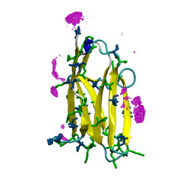
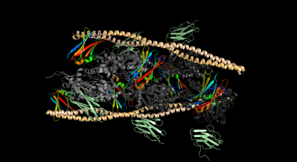
The simulated C1 protein is a subunit of MyBPC, which itself is part of the myosin thin filament. The filament (image shown below) contains tropomyosin (pale orange), filamentous actin (grey), troponin (not shown), and the MyBPC protein (C1 shown colored by rainbow and C0 shown colored green and other CX subunits not “crystallized”). As several cryo-EM based all-atom structures of this filament exists (PDB: 6cxi) it would be helpful to understand the C1 ion density as a function of the entire thin filament’s structure.

Calculating Ion Density with CPPTRAJ

What we want to do is take the ion density calculated for each C1 monomer trajectory and map it onto the large filament. First we will determine an appropriate grid size. Then we will fit the C1 monomer onto each subunit of the large filament (using the PDB of the filament as a reference). Then we will calculate the ion density on the grid, ensuring the grid is fit to the C1 monomer.

Determine Grid Dimensions

We want to ensure the grid we use is large enough to capture ion density around the C1 monomer. We can use the bounds command to do this.

1. Read some of the C1 trajectory information in with trajin to define the grid spacing which covers the protein. It should be a significant amount of trajectory information to ensure we have a good idea of how much the protein moves; I am using 5 microseconds in this example.
2. We will RMS-best-fit the C1 monomer onto a subunit of the filament using the rms command, so we need to read in the filament PDB as a reference. We will also calculate the coordinate RMSD to check our fitting (rmsd.G.dat)
3. We will use the bounds command to find the extent to which the C1 monomer moves in the X, Y, and Z dimensions. We will also determine what dimensions to use for a grid using a 0.5 Angstrom spacing around all protein residues, along with a small buffer zone.
4. Once the bounds command is run, the output information in the will include the number of bins in each dimension which cover the protein (rmsd.G.dat)

# Load simulation topology file.
parm nowat.C1_Cu2ions.parm7
# Load reference topology and structure.
parm ../6cxi.pdb
reference ../6cxi.pdb parmindex 1
# Load simulation trajectory.
# 1 trajectory should be enough to determine bounds for grid.
trajin ~/run.C1_Cu2/analysis/nowat.withions.nc.0
# Fit simulation to reference.
# Target residues 31-34 (original ref 181-184)
# are not present in chain G.
rms reference :1-30,35-108@CA ::G&@CA out rmsd.G.dat
# Get the extent of the protein (residues 1 to 108) to
# determine grid size. Add an offset of 8 bins in each
# dimension.
bounds :1-108 out bounds.G.dat name GridG dx 0.5 offset 8
run

Here are the results from the ‘bounds’ command for the C1 monomer after being fit onto a subunit of the filament reference PDB:

$ head bounds.G.dat

-42.883701 < X < 15.029673       Center= -13.927014  Bins=124
 13.966270 < Y < 66.035890       Center= 40.001080  Bins=113
 37.514960 < Z < 84.779227       Center= 61.147093  Bins=103

You can see from the results that the largest number of bins is in the X dimension with 124. It is very close to the other values, so we can round up to 124 for Y and Z to make the grid cubic (although this is not technically necessary, having a uniform grid can be beneficial if e.g. the protein tends to change its shape during the simulation). It is important to not choose the lowest dimension, or you may leave out meaningful data.

Calculating Ion Density

Now that we know how big to make the grid dimensions in order to capture ion density around our C1 monomer trajectories, we can fit each trajectory (with ion information) to a specific subunit of the filament (over the six subunits using a ‘for’ loop), and calculate the ion density on the grid.

1. Round up the number of bins from bounds.G.dat in each dimension to make the grid cubic (124 in our example).
2. Read in the filament PDB as a reference structure, and trajectory with its topology (6cxi.pdb, nowat.withions.nc, nowat.withions.parm7).
3. Now we set up a ‘for’ loop so we can have our trajectory with ions fit to a specific chain of the larger filament. The six C1 subunits in the 6cxi PDB are denoted by chain IDs G, H, I, J, K, and L.
   1. Inside the loop, we rms fit the trajectory data (with ions) to the specific chain.
   2. Then we grid the Cu²⁺ ions, using a 0.5 Angstrom grid spacing and setting the bounds of the grid to be the number of bins from the previous CPPTRAJ run (bounds.G.dat).
   3. Last, an average structure from trajectory frames is printed out to make sure the fit made sense (average.G.mol2) and for visualization.
4. The for loop (and program) ends after repeating for all chains specified, and we have the following output files:

avg.G.mol2, avg.H.mol2, avg.I.mol2, avg.J.mol2, avg.K.mol2, avg.L.mol2, bounds.G.dat, Grid.G.dx, Grid.H.dx, Grid.I.dx, Grid.J.dx, Grid.K.dx, Grid.L.dx, rmsd.G.dat, rmsd.H.dat, rmsd.I.dat, rmsd.J.dat, rmsd.K.dat, rmsd.L.dat

# Load simulation topology file.
parm nowat.C1_Cu2ions.parm7
# Load reference topology and structure.
parm ../6cxi.pdb
reference ../6cxi.pdb parmindex 1
# Load simulation trajectory.
trajin ~/run.C1_Cu2/analysis/nowat.withions.nc.0
# Loop over subunit chains in reference.
for CID in G,H,I,J,K,L
# Fit to simulation to reference subunit.
# Target residues 31-34 (original ref 181-184)
# are not present in target chain.
rms R.$CID reference :1-30,35-108@CA ::$CID&@CA out rmsd.$CID.dat
# Grid CU density, fit grid on the subunit residues.
# Use Bins from bounds output to set up grid size.
# No need to X-align the grid since DX format
# supports non-X-aligned grids.
grid :CU out Grid.$CID.dx name Grid$CID \
rmsfit :1-108@CA noxalign normframe \
124 0.5 124 0.5 124 0.5
# Calculate average structure, write to file.
average avg.$CID.mol2 :1-108
done
run

Visualizing the results (in VMD)

We want to visualize the density on the 6cxi intact filament structure, so let’s open that in VMD (6cxi.pdb).

File -> New Molecule -> Browse… (to 6cxi.pdb), then Load.

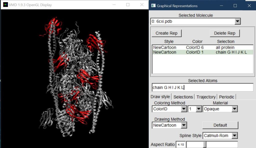
To highlight the C1 protein, we put everything in New Cartoon representation, and create a new representation for chains G through L and choose a bright color.

Next, we go to File -> New Molecule and open up the Molecule File Browser.

Browse for the Grid.G.dx files, select the DX file type if it does not automatically determine this based on the “.dx” extension, and Load. A box should appear over the Chain G protein. Colored chain G yellow here to highlight it.

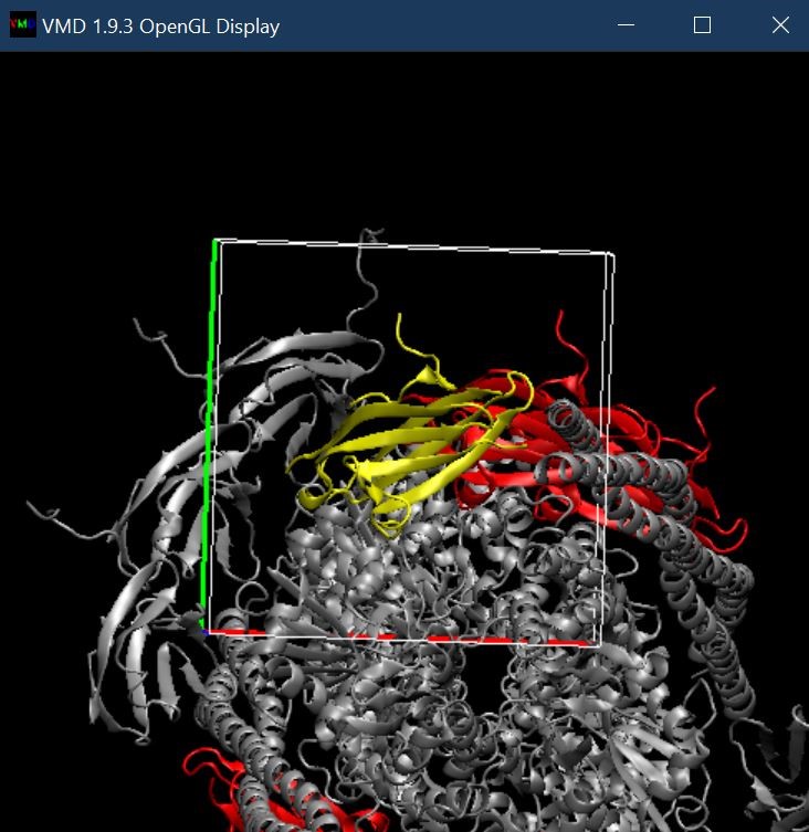
Next, in the Grid.G.dx representation, select the range and isovalues that yield the percentage distribution of ions you want to visualize. Representation is into a Solid Surface and choose a highlighting color (cyan2). Here, the range is 0 to 0.004 and the isovalue is 0.0006 – this means the density is 15% of bulk.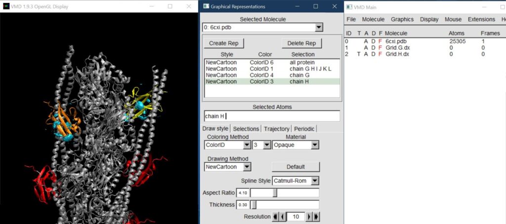

Repeat the previous two steps for the Grid.H.dx file (step 1 = File -> New Molecule -> Browse for Grid.H.dx; step 2 = adjust range and isovalue to match Grid.G.dx and change representation). Below, chain H is highlighted in orange, chain G is in yellow, and the 15% over bulk density of Cu²⁺ is shown on each chain as a cyan surface.

Continue opening up Grid.X.dx files as New Molecules until all chains have been added.

For a “shortcut,” once you set up the first grid’s representation and isovalue/ranges, you can use (VMD Main window) Extensions -> Visualization -> Clone Representation to clone the representation to the rest of the grids.

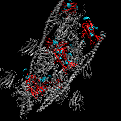
The result will look like the following figure.

For clarity, we can put the actin in QuickSurface Drawing method and the tropomyosin in a different color, and hide the C0 subunits:

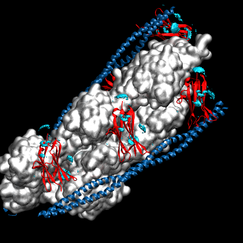
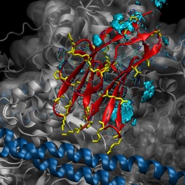
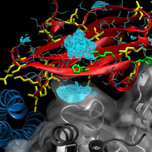
To solve our initial question about where Cu²⁺ density is located, and might that affect actin binding, we need to take a closer look at the structure. Below is a close-up on C1 Chain I with its gridded Cu²⁺ density, tropomyosin in blue, and the three actin proteins in shades of grey. There is significant density between one of the actin-C1 faces, coordinated around histidine residues on neighboring beta strands. This density could potentially disrupt binding, but we should keep a few things in mind: 1) the density was modeled using the individual C1 subunit – we do not know for sure this same ion binding would occur once C1 binds tropomyosin and actin to make the thin filament. 2) The model of the filament is based on coarse grain data from Cryo-EM. The C1 subunit fits the density, but we do not know that this is ultimately the correct, or only, conformation in which it binds. Nonetheless, the simulations have generated a testable hypothesis – perhaps we can control Cu²⁺ binding by modulating pH and controlling HIS protonation, or incorporate point mutations to get rid of HIS residues, and abolish Cu²⁺ binding sites in C1.