
CPPTRAJ is the main program in AMBER for processing coordinate trajectories and data files.
The program CPPTRAJ, included in AmberTools, is a new and rewritten version of the historical PTRAJ program developed by Prof. Thomas E. Cheatham III, at the University of Utah. CPPTRAJ is at least as fast as PTRAJ was, and is in many cases significantly faster, and offers multiple option for analysis and trajectory processing of Molecular Dynamics data in multiple formats. For more information about CPPTRAJ, there are two published articles in JCTC and JCC
If in interactive mode, the help command can be used to list recognized commands and topics; topics (such as mask syntax) start with uppercase letters. help <command> can be used to get the associated keywords as well as an abbreviated description of the command. Most commands have a corresponding test which also serves as an example of how to use the command. See $AMBERHOME/AmberTools/test/cpptraj/README for more details.
In this introduction, we present a brief overview of analyzing simulation data with CPPTRAJ. Some basic and common types of analysis will be covered, as well as the basics of data set handling in CPPTRAJ. This assumes that AmberTools has been successfully installed and has been tested. This also assumes some familiarity with AMBER atom mask selection syntax. In addition, xmgrace will be required to view some of the output data.
Throughout this tutorial a short example trajectory of the beta-hairpin trpzip2 will be used. The trajectory is in NetCDF format, which is faster to process, more compact, higher precision, and more robust than the ASCII format. NetCDF is enabled by default in AMBER. The trajectory and associated topology can be downloaded here:
trpzip2.ff10.mbondi.parm7 — This is the topology file.
trpzip2.gb.nc — This is the trajectory file.
A movie of the trajectory of the beta-hairpin trpzip2 is presented below:
Loading a Topology and Trajectory
To start CPPTRAJ, type cpptraj from the command line:
[user@computer ~]$ cpptraj
CPPTRAJ: Trajectory Analysis. V5.0.4 (GitHub)
___ ___ ___ ___ __
 | \/ | \/ | \/ |
_|_/\_|_/\_|_/\_|_

| Date/time: 11/03/23 16:02:12
| Available memory: 10.203 GB
Running CPPTRAJ with no arguments brings up the interactive command line. The command line is useful for running simple or short analyses. The command line allows tab completion of file names and commands. Also, in interactive mode all commands used are written to the file ‘cpptraj.log’ (this name can be changed with the ‘–log ‘ command line switch). Before reading in a trajectory, CPPTRAJ needs to know what the system looks like. This information is contained with topology files. The first step is to load the topology file with the parm command:
> parm trpzip2.ff10.mbondi.parm7
   [parm trpzip2.ff10.mbondi.parm7]
   Reading 'trpzip2.ff10.mbondi.parm7' as Amber Topology
   Radius Set: modified Bondi radii (mbondi)
   This Amber topology does not include atomic numbers.
   Assigning elements from atom masses/names.
   No SCEE section: setting Amber default (1.2)
   No SCNB section: setting Amber default (2.0)
The topology has now been loaded. You can see what topologies are loaded with the list command:
> list parm
   [list parm]

   PARAMETER FILES (1 total):
   0: trpzip2.ff10.mbondi.parm7, 220 atoms, 13 res, box: None, 1 mol
The output shows the topology index (which starts from 0, depicted in red here) followed by some brief information on the topology. More detailed information can be obtained using the ‘parminfo <#>’ command, where <#> is the index of the desired topology:
> parminfo 0
   [parminfo 0]    Topology trpzip2.ff10.mbondi.parm7 contains 220 atoms.
   Original filename: trpzip2.ff10.mbondi.parm7
   13 residues.
   1 molecules.
   227 bonds (104 to H, 123 other).
   402 angles (233 with H, 169 other).
   853 dihedrals (481 with H, 372 other).
   Box: None
   GB radii set: modified Bondi radii (mbondi)
Now that the topology file is loaded, we can tell CPPTRAJ which trajectory we are going to process, we use the command trajin:
> trajin trpzip2.gb.nc
   [trajin trpzip2.gb.nc]
   Reading 'trpzip2.gb.nc' as Amber NetCDF
   Warning: NetCDF file time variable defined but empty. Disabling.
Note that this does not immediately read the trajectory, rather it places the trajectory in the input trajectory list for processing later. To see what trajectories are currently in the input trajectory list we can again use the list command:
> list trajin
   [list trajin]

   INPUT TRAJECTORIES (1 total):
   0: 'trpzip2.gb.nc' is a NetCDF AMBER trajectory with coordinates, Parm trpzip2.ff10.mbondi.parm7 (reading 1201 of 1201)
   Coordinate processing will occur on 1201 frames.
Specifying an Action
Now that a topology and trajectory have been loaded, we can specify actions to generate data from the trajectory. Say for example we would like to know the end-to-end distance for the hairpin over the course of the trajectory. We can use the distance command to get this information. First, we can use the help command to remind us of the syntax for distance:
> help distance
   [help distance]
   [<name>] <mask1> [<mask2>] [point <X> <Y> <Z>]
   [ reference | ref <name> | refindex <#> ]
   [out <filename>] [geom] [noimage] [type noe]
   Options for 'type noe':
   [bound <lower> bound <upper>] [rexp <expected>] [noe_strong] [noe_medium] [noe_weak]
   Calculate distance between atoms in <mask1> and <mask2>, between
   atoms in <mask1> and atoms in <mask2> in specified reference, or
   atoms in <mask1> and the specified point.
The help command can be used with no arguments to bring up a list of all commands. In order to figure out which atoms correspond with the end residues of trpzip2, we can use the resinfo command:
> resinfo
[resinfo]
13 residues selected.
#Res Name First Last Natom #Orig #Mol C I
   1 SER  1     13   13    1     1
   2 TRP  14    37   24    2     1
   3 THR  38    51   14    3     1
   4 TRP  52    75   24    4     1
   5 GLU  76    90   15    5     1
   6 ASN  91    104  14    6     1
   7 GLY  105   111  7     7     1
   8 LYS  112   133  22    8     1
   9 TRP  134   157  24    9     1
  10 THR  158   171  14    10    1
  11 TRP  172   195  24    11    1
  12 LYS  196   217  22    12    1
  13 NHE  218   220  3     13    1
From this output we can see that our end residues are 1 and 13. In general, the resinfo, atominfo, and molinfo commands are useful for examining your system layout and/or testing the result of an atom mask expression. For example, to see what atoms will be selected by the atom mask :13 (residue 13):
> atominfo :13
   [atominfo :13]
   3 atoms selected.
   #Atom Name #Res Name #Mol Type Charge  Mass    GBradius El rVDW   eVDW
   218   N    13   NHE  1    N    -0.4630 14.0100 1.5500   N  1.8240 0.1700
   219   HN1  13   NHE  1    H    0.2315   1.0080 1.3000   H  0.6000 0.0157
   220   HN2  13   NHE  1    H    0.2315   1.0080 1.3000   H  0.6000 0.0157
We can now enter our distance command:
> distance end-to-end :1 :13 out dist-end-to-end.agr
   [distance end-to-end :1 :13 out dist-end-to-end.agr]
   DISTANCE: :1 to :13, center of mass.
This says to calculate a distance named end-to-end from the center of mass of residue 1 to residue 13, writing the results to a file named dist-end-to-end.agr. The file format will be xmgrace-readable because the filename extension ‘.agr’ is recognized by CPPTRAJ as xmgrace. We could change the format to gnuplot-readable by specifying a ‘.gnu’ extension instead. If the extension is ‘.dat’ or not recognized, CPPTRAJ will default to a standard column format. The supported formats and their options are listed here. Note that similar to trajin, entering an action does not execute it right away. Instead, it has gone into the action list. To see what actions are currently present in the action list we can use the list command:
> list actions
   [list actions]

   ACTIONS (1 total):
   0: [distance end-to-end :1 :13 out dist-end-to-end.agr]
Processing the Trajectory
We have now loaded a topology, a trajectory, and have specified an action. The command can now be executed by specifying ‘run’ or ‘go’. This tells CPPTRAJ to process each loaded trajectory, executing any specified actions on each frame. During trajectory processing some information will be printed that describes what CPPTRAJ is doing. First, information on the currently loaded topologies and trajectories are printed:
> run
[run]
---------- RUN BEGIN -------------------------------------------------

PARAMETER FILES (1 total):
0: trpzip2.ff10.mbondi.parm7, 220 atoms, 13 res, box: None, 1 mol

INPUT TRAJECTORIES (1 total):
0: 'trpzip2.gb.nc' is a NetCDF AMBER trajectory with coordinates, Parm trpzip2.ff10.mbondi.parm7 (reading 1201 of 1201)
Coordinate processing will occur on 1201 frames.

BEGIN TRAJECTORY PROCESSING:
.....................................................
ACTION SETUP FOR PARM 'trpzip2.ff10.mbondi.parm7' (1 actions):
0: [distance end-to-end :1 :13 out dist-end-to-end.agr]
:1 (13 atoms) to :13 (3 atoms), imaging off.
----- trpzip2.gb.nc (1-1201, 1) -----
0% 10% 20% 30% 40% 50% 60% 70% 80% 90% 100% Complete.

Read 1201 frames and processed 1201 frames.
TIME: Avg. throughput= 106217.3875 frames / second.

ACTION OUTPUT:
TIME: Analyses took 0.0000 seconds.

DATASETS (1 total):
end-to-end "end-to-end" (double, distance), size is 1201 (9.608 kB)
Total data set memory usage is at least 9.608 kB

DATAFILES (1 total):
dist-end-to-end.agr (Grace File): end-to-end

RUN TIMING:
TIME: Init : 0.0000 s ( 0.23%)
TIME: Trajectory Process : 0.0113 s ( 82.68%)
TIME: Action Post : 0.0000 s ( 0.01%)
TIME: Analysis : 0.0000 s ( 0.01%)
TIME: Data File Write : 0.0023 s ( 16.90%)
TIME: Other : 0.0000 s ( 0.00%)
TIME: Run Total 0.0137 s
---------- RUN END ---------------------------------------------------
After CPPTRAJ finishes the analysis, you can exit CPPTRAJ typing quit:
> quit
[quit]
--------------------------------------------------------------------------------
To cite CPPTRAJ use:
Daniel R. Roe and Thomas E. Cheatham, III, "PTRAJ and CPPTRAJ: Software for
Processing and Analysis of Molecular Dynamics Trajectory Data". J. Chem.
Theory Comput., 2013, 9 (7), pp 3084-3095.
You should have an xmgrace file (with the name dist-end-to-end.agr) that you can open with xmgrace:
[user@computer ~]$ xmgrace dist-end-to-end.agr
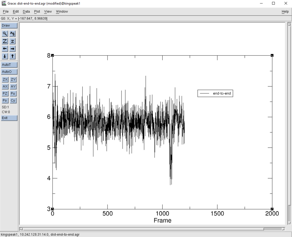
This shows a plot of the distance (in Angstroms) between the first residue and residue number 13 (as per the mask used of :1 :13). The frame number in the X axis translates to the simulation time.
Next we recommend a tutorial on working with Data Sets following this link (Introduction to Data Sets).