Making a 3d histogram of the position of a small molecule around a receptor.
You want to see where a ligand is spending more time around a receptor.
When you have a ligand that is exploring multiple binding positions, sometimes is useful to visually see where it is spending more time. A qualitatively way of doing this is using the grid command of CPPTRAJ to bin the ligand into a 3D grid. For this recipie, we are going to use a simulation between the compound berenil interacting with a 15 residue DNA folded into a g-quadruplex. The simulation is 400 ns long performed with the OL15 force field in AMBER.
You can see that the ligand is mainly populating two positions on both sides of the g-quadruplex. In order to qualitatively see where it is spending more time, we can use a combination of commands available in CPPTRAJ to create a 3D representation of the positions of the ligand. The overall steps are: reading the topology and trajectory files, reorienting the solute and fitting the frames, generating a boundary box where the analysis is going to be performed (in this case, around the DNA g-quadruplex) and with this information, generate a a 3D histogram of the berenil ligand.
It is very important to make sure that the trajectory data has been reoriented and centered using the autoimage command and has been rms fitted in order to provide a meaningful representation.
We are going to use the bounds command to calculate the boundaries that the ligand is exploring. We need to do this in order to tell the grid command where to set the bounding box to perform the analysis
The CPPTRAJ input is:
parm nowater.parm7
trajin nowater.nc
autoimage
rms fit :1-15&!@H= mass
bounds :1-15 dx 0.5 name MyGrid out boundaries.dat
 average average.pdb pdb :1-15
createcrd MyCoords

run

crdaction MyCoords grid ligand-grid.xplor data MyGrid :16
The DNA residues are from 1 to 15 and the berenil ligand is residue id 16. We use the command parm to read the topology and trajin to read the trajectory file. Then we use autoimage to re-orient the molecules and we perform a root mean square fit with rms. The mask for the rms command includes the DNA residues 1 to 15 and does not include hydrogen atoms. The fit will be based on the mass of the atoms. For the bounds command, we are going to calculate the boundaries of just the g-quadruplex by selecting residues 1 to 15. If we calculate the boundaries including the ligand, the box will be bigger in order to accommodate those events where the ligands is far from the DNA, and we do not want to include those events. The dx 0.5 tells the command that the spacing will be every 0.5 in the three x, y and z directions. The result of the bounds command will be saved internally with the name ‘MyGrid’, and the same data will be saved to a file with the name boundaries.dat. The contents of this file are:
12.138568 < X < 47.525350 Center= 29.831959 Bins=72
9.558702 < Y < 44.375636 Center= 26.967169 Bins=71
11.444081 < Z < 43.796951 Center= 27.620516 Bins=66
This information sets the boundaries for x, y and z, the center and the number of bins to use. This information will be used by the grid command. Next step is creating an average structure with the average command focusing only on residues 1 to 15 and saving the average as a pdb file with the name average.pdb. Now we create a data set with coordinates using the name ‘MyCoords’ that will store the trajectory information. We now execute the commands so far with the keyword run . At this time, we have the boundaries information, our average structure and all the trajectory information under the dataset ‘MyCoords’.
Next step, we are going to use the crdaction command to perform the grid analysis in the data saved in ‘MyCoords’.
crdaction MyCoords grid ligand-grid.xplor data MyGrid :16
This command uses the crdaction keyword to apply an action to the information stored in ‘MyCoords’. The action to apply is the grid command, which will save the grid with the name ligand-grid.xplor using the XPLOR format and the data to read the information regarding the bins and center is in the MyGrid dataset, calculated previously. The residue id that the grid command is going to use is 16, which corresponds to the berenil ligand.
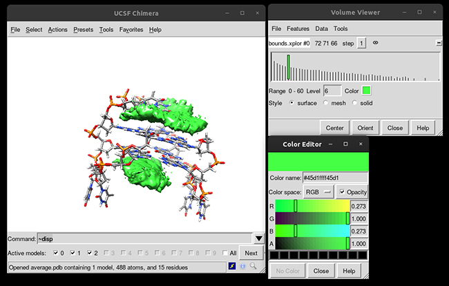
Running the script will generate the average.pdb structure, the boundaries.dat file with the boundaries information and the ligand-grid.xplor file with the 3D information. Using UCSF-Chimera, we can go to Tools -> Volume data -> Volume Viewer.
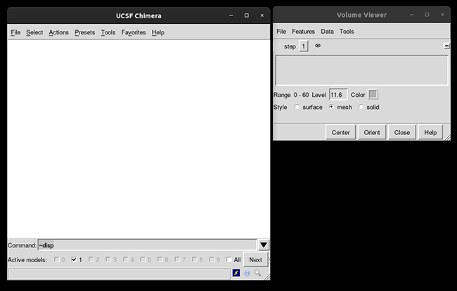
In the Volume viewer window, go to File -> Open map and load the ligand-grid.xplor file.
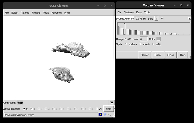
This will load your explore data as a solid surface. Now we load the average structure to provide some reference.
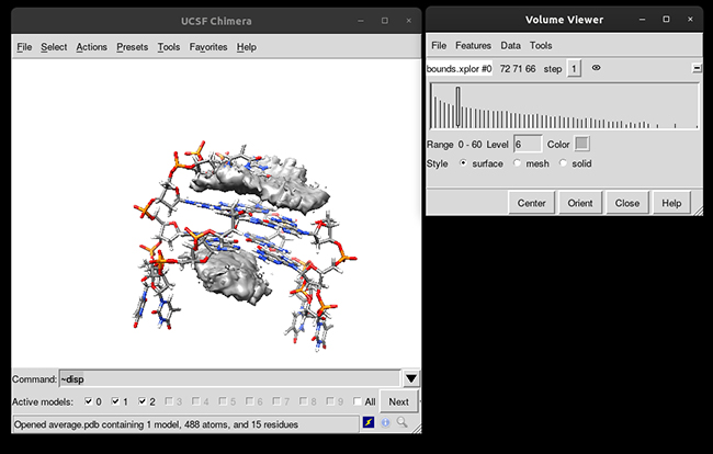
You can see that the g-quadruplex average structure is between the two grid volumes that we calculated. There are multiple options available to change the isodensity value, the range, the style and even the color of the calculated grid:
This analysis was able to provide to us a quantitatively form of studying the different binding modes that a ligand can have in a receptor and helps to suggest further analysis.