
Clustering a protein from multiple independent copies
You need to extract a representative structure from three independent runs of a protein simulation.
In this example, we will use the 575 amino acid tyrosine phosphatase from the PDB code 1LAR. We have included an inhibitor in the active site of the enzyme using docking and homology tools. We want to detect the conformational changes produced by the ligand after running molecular dynamics simulations. To increase the sampling time in order to reach convergence, we have run three independent simulations. These independent simulations each run in its own GPU node using pmemd.cuda from AMBER and they all started from the same restart file that was generated in a previous step after exhaustive minimization, heating and equilibration time. The practice of running multiple independent copies of the same system is currently a necessary practice when doing MD simulations in order to provide robust data that yield more accurate results and hence are more in-tune with experimental observations.
The topology file is 1lar-nowater.parm7 and the three runs are 1lar-nowater-run1.nc, 1lar-nowater-run2.nc and 1lar-nowater-run3.nc, each has been run for ~3 microseconds. These are big files (~ 1.7 GB each), so they could take some time to download. The water has been deleted from the topology file (using parmstrip) and from the trajectories (using strip). The trajectories have also been autoimaged and rms fitted to the protein (see this recipe). Also, to save space, the trajectory was reduced to every 10th frame. The total number of frames for each trajectory is:
cpptraj -p 1lar-nowater.parm7 -y 1lar-nowater-run1.nc -tl
Frames: 15477
cpptraj -p 1lar-nowater.parm7 -y 1lar-nowater-run2.nc -tl
Frames: 16635
cpptraj -p 1lar-nowater.parm7 -y 1lar-nowater-run3.nc -tl
Frames: 15711
To calculate the sampling time, we multiply the number of frames times how frequent we saved the trajectory data (ntwx=5 000) times the time step used (0.004). This gives for 1lar-nowater-run1.nc = 15 477 x 5 000 x 0.004 = 309 540 ps, but remember that we only saved every 10th frame to save space, so 309 540 x 10 = 3 095 400 ps, which corresponds to 3.09 microseconds.
How can we extract a representative structure from our simulation data? One way of determining structure populations from simulations is cluster analysis. Clustering is a means of partitioning data so that data points inside a cluster are more similar to each other than they are to points outside a cluster. In the context of molecular simulation, this means grouping similar conformations together. Similarity is determined by a distance metric – the smaller the distance, the more similar the structures. One commonly used distance metric is coordinate RMSD.
It is very important to note that there is no one “correct” way to perform cluster analysis. There are many different algorithms and distance metrics available, and different combinations will work better for certain systems. Cluster analysis usually requires some trial and error before satisfactory results are obtained. For a more in-depth discussion on cluster analysis of MD trajectories, users are encouraged to read the 2007 paper by Shao et al. on the subject.
We will test three clustering algorithms available in CPPTRAJ (k-means, dbscan and hierarchical agglomerative) available in the cluster command in order to understand the differences and see which algorithm could provide more information for our system. Again, please refer to the article by Shao for further details and differences of each method.
K-means clustering algorithm.
The CPPTRAJ input script that we will use looks like this:
parm 1lar-nowater.parm7
trajin 1lar-nowater-run1.nc 1 last 10
trajin 1lar-nowater-run2.nc 1 last 10
trajin 1lar-nowater-run3.nc 1 last 10
strip :Na+,Cl-
cluster c1 \
 kmeans clusters 10 randompoint maxit 500 \
   rms :1-576@C,N,O,CA,CB&!@H= \
   sieve 10 random \
 out cnumvtime.dat \
  summary summary.dat \
  info info.dat \
  cpopvtime cpopvtime.agr normframe \
  repout rep repfmt pdb \
  singlerepout singlerep.nc singlerepfmt netcdf \
  avgout avg avgfmt pdb
 run
Each step consist of:
parm 1lar-nowater.parm7– Reads the topology.trajin 1lar-nowater-run1.nc 1 last 10– Will read the trajectory file starting from frame 1 until the last frame, and skipping every 10th frame. We will skip every 10th frame to speed up the calculations. We include this command for each of the trajectory files.strip :Na+,Cl-– Will delete the ions that are present in both the topology and the trajectory data.cluster c1– calls the cluster command and sets the data set name.kmeans– use the kmeans clustering algorith.clusters 10– Finish clustering when number of clusters is 10.randompoint– Randomize initial set of points used.maxit 500– Algorithm will run until frames no longer change clusters of 500 iterations are reached.rms :1-576@C,N,O,CA,CB&!@H=– Use the RMSD of residues 1 to 576 and only using atoms C, N, O, CA and CB as distance metric, do not consider hydrogens.sieve 10 random– Typically generating the pair-wise distance matrix (the distance of every frame to every other frame) is a very time and memory consuming part of the clustering calculation. “Sieving” is a way to reduce the expense of this step by using “total / 10” frames for initial clustering. The sieved frames are then added to those clusters as an additional step.randommakes the sieve random, instead of ordered.out cnumvtime.dat– Write cluster number versus time to a file with the name cnumvtime.dat.summary summary.dat– Write overall clustering summary to summary.datinfo info.dat– Write detailed cluster results (including DBI, pSF etc) to info.dat.cpopvtime cpopvtime.agr normframe– Write cluster population vs time to ‘cpopvtiime.agr’, normalized by # frames. The ‘agr’ file is an XMGRACE plot.repout rep repfmt pdb– Write cluster representative structure to ‘repX’ with PDB format, where X is the cluster number.singlerepout singlerep.nc singlerepfmt netcdf– Write all cluster representatives to ‘singlerep.nc’ with NetCDF format.avgout avg avgfmt pdb– Write average over all frames in each cluster to files starting with ‘avg’ using PDB as the file format.
Running this script will read the three independent trajectory files (every 10th frame) and create 10 clusters using a total number of 4784 frames. The summary file looks like this:
#Cluster Frames Frac  AvgDist Stdev Centroid AvgCDist
0          1092 0.228 2.199   0.507     4133    8.709
1           890 0.186 2.146   0.400     3029    6.296
2           767 0.160 2.337   0.464     2036    6.331
3           615 0.129 2.459   0.508      644    6.037
4           430 0.090 2.470   0.623     3550    8.148
5           343 0.072 2.083   0.328     1291    6.767
6           314 0.066 2.471   0.507      262    6.478
7           243 0.051 2.050   0.469     1042    6.362
8            58 0.012 3.788   1.180     3221    7.082
9            32 0.007 2.387   0.000       26    7.467
The most populated cluster (#0) includes 1092 frames which represents 22.8% of the total processed frames. The average distance between points in the cluster for cluster #0 is 2.199 (with 0.507 of standard deviation). In frame 4133 we can find the structure that has the lowest cumulative distance to every other point and the average distance of this cluster to every other cluster is 8.7 angstroms.
Hierarchical agglomerative (bottom-up) algorithm.
The CPPTRAJ input script that we will use looks like this:
parm 1lar-nowater.parm7
trajin 1lar-nowater-run1.nc 1 last 10
trajin 1lar-nowater-run2.nc 1 last 10
trajin 1lar-nowater-run3.nc 1 last 10
strip :Na+,Cl-
cluster c1 \
  hieragglo epsilon 3.0 clusters 10 averagelinkage \
  rms :1-576@C,N,O,CA,CB&!@H= \
  sieve 10 random \
  out cnumvtime.dat \
  summary summary.dat \
  info info.dat \
  cpopvtime cpopvtime.agr normframe \
  repout rep repfmt pdb \
  singlerepout singlerep.nc singlerepfmt netcdf \
  avgout avg avgfmt pdb
run
The input is very similar to the one we used for K-means. The difference is in the cluster line:
hieragglo epsilon 3.0 clusters 10 averagelinkage– This sets the use of the hierarchical agglomerative (bottom-up) approach. Clustering will finish when a minimum distance between clusters is greater than 3, Finish clustering when 10 clusters remain and we will use average-linkage that uses the average distance between members of two clusters.
The rest of the input file is the same. In this case, the summary file is:
#Cluster Frames Frac  AvgDist Stdev Centroid AvgCDist
0          1656 0.346   2.672 0.551     2411    7.340
1          1073 0.224   2.142 0.471     4133    8.937
2           488 0.102   2.454 0.530      219    7.089
3           461 0.096   2.257 0.460      680    7.023
4           347 0.073   2.245 0.440     1306    7.768
5           280 0.059   2.273 0.629     3421    8.320
6           205 0.043   1.898 0.368     1103    7.415
7           172 0.036   2.006 0.489     3636    8.696
8            44 0.009   2.067 0.000     3230    7.443
9            22 0.005   2.270 0.507       35    7.599
10           18 0.004   0.000 0.000       11    7.261
11           12 0.003   0.000 0.000     1550    7.421
12            6 0.001   0.000 0.000       17    9.671
We can see that even though we set clusters to 10, the algorithm produced 13 total clusters, but with very low populations.
DBScan clustering algorithm.
When using dbscan, it is necessary to set the values for the minimum # of points to form a cluster (minpoints) and the distance cutoff for forming cluster (epsilon). A rough idea can be obtained by generating a ‘K-dist’ plot that will show for each frame (X axis) the Kth farthest distance (Y axis), sorted by decreasing distance. We can calculate the K-dist plot using the CPPTRAJ input:
parm 1lar-nowater.parm7
trajin 1lar-nowater-run1.nc 1 last 10
trajin 1lar-nowater-run2.nc 1 last 10
trajin 1lar-nowater-run3.nc 1 last 10
strip :Na+,Cl-
cluster c1 dbscan kdist 1 rms :1-576@C,N,O,CA,CB&!@H=
cluster c2 dbscan kdist 2 rms :1-576@C,N,O,CA,CB&!@H=
cluster c3 dbscan kdist 3 rms :1-576@C,N,O,CA,CB&!@H=
cluster c4 dbscan kdist 4 rms :1-576@C,N,O,CA,CB&!@H=
cluster c5 dbscan kdist 5 rms :1-576@C,N,O,CA,CB&!@H=
cluster c6 dbscan kdist 6 rms :1-576@C,N,O,CA,CB&!@H=
run
This CPPTRAJ input will run a cluster command six times using six different value for the kdist option, and with each command an individual Kdist file is generated (Kdist.1.dat to Kdist.6.dat). Again, the Kdist analysis will be performed in residues 1 to 575, only considering the atom types C, N, O, CA and CB, and no hydrogens will be considering. Plotting the six resulting files renders:
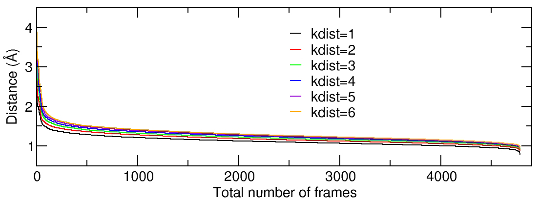
We can see from the plot that we have a steep slope initially and the curves begin to flatten out at ~2.0 angstroms. There is no significant difference between the kdist value and It has been suggested that the shape of the K-dist curve doesn’t change too much after Kdist=4, so we will use a value of 4 for minpoints and an epsilon value of 2. The CPPTRAJ input looks like:
parm 1lar-nowater.parm7
trajin 1lar-nowater-run1.nc 1 last 10
trajin 1lar-nowater-run2.nc 1 last 10
trajin 1lar-nowater-run3.nc 1 last 10
strip :Na+,Cl-
cluster c0 \
      dbscan minpoints 4 epsilon 2.0 sievetoframe \
      rms :1-576@C,N,O,CA,CB&!@H= \
      sieve 10 random \
      out cnumvtime.dat \
      summary summary.dat \
      info info.dat \
      cpopvtime cpopvtime.agr normframe \
      repout rep repfmt pdb \
      singlerepout singlerep.nc singlerepfmt netcdf \
    avgout avg avgfmt pdb
run
We now incorporate the minpoints and epsilon values to the input for the dbscan algorithm and include the same output options as with the previous examples.
Comparison of the Various Clustering Algorithms Applied to three independent trajectory information, each ~15k frames long, corresponding to ~3 microseconds. In the info.dat file in each analysis we can find the values of DBI, pSF and SSR/SST. The DBI and psF values are metrics of clustering quality; low values of DBI and high values of pSF indicate better results. The R-squared (SSR/SST) value represents the percentage of variance explained by the data. More information is available in the cluster entry of the manual and the Shao article.
| Algorithm | DBI | pSF | SSR/SST | Cluster size | Run total (seconds) |
| dbscan | 1.1278 | 5879.27 | 0.8850 | 1633,1096,784,423 | 29.0 |
| k-means | 1.2641 | 4596.00 | 0.8965 | 1092,890,767,615 | 20.6 |
| hierarchical | 1.2677 | 3223.47 | 0.8902 | 1656,1073,488,461 | 20.6 |
We can see from the data that the three algorithms used perform very similar. Low DBI values and high pSF values signal better clustering. The cluster size for the first four most populated clusters are very similar for dbscan and hierarchical. We could think that dbscan is somewhat more appropriate for this particular dataset, although it takes more time to process as we can see from the ‘Run total’ column that could be an issue in bigger trajectories.
One particularly interesting output are the cluster populations versus time, written to ‘cpopvtime.agr’.
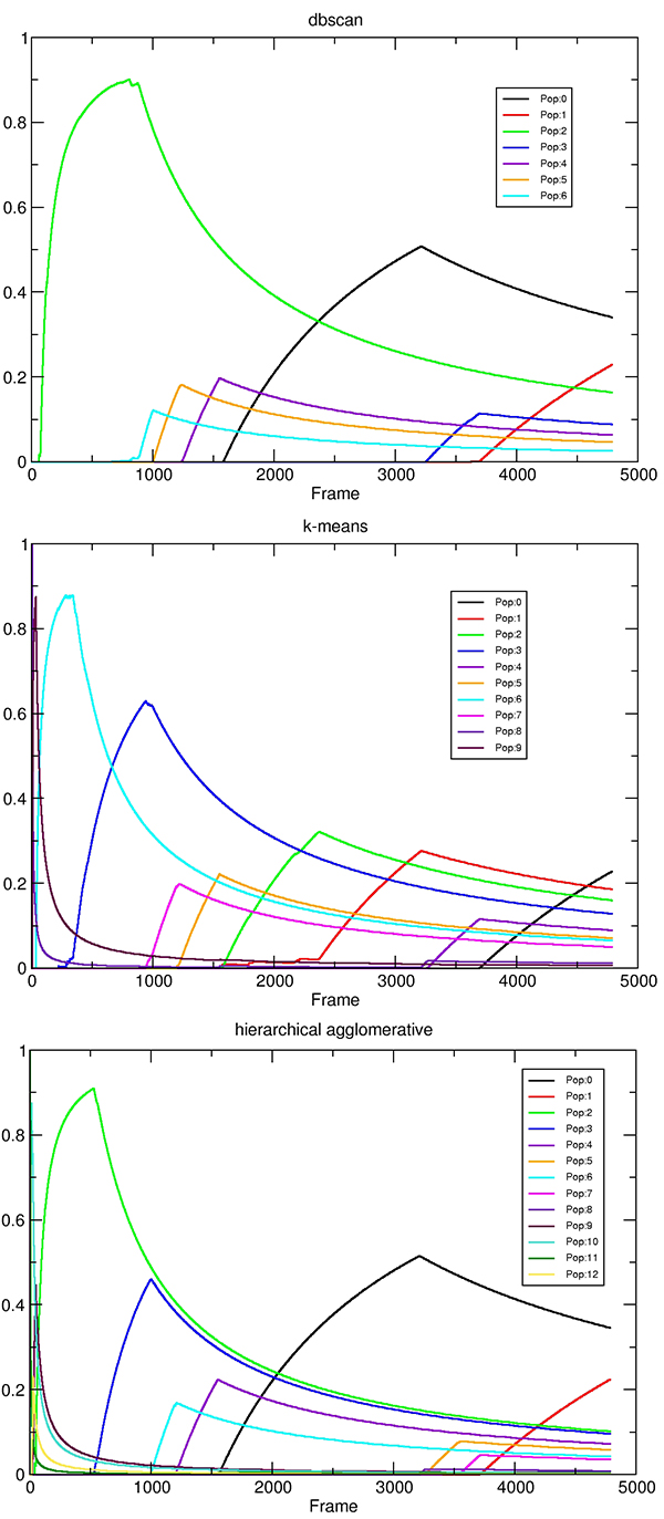
In particular one can see that at the beginning of the trajectory the cluster populations are changing rapidly over time. As the run progresses the cluster populations gradually stabilize until they reach their final values at 4780 frames (the total number of frames of the three independent trajectories). This is an indication that the cluster populations are reaching an equilibrium and the results may be suitable for things like thermodynamic analysis. We can also see the similarities with the dbscan and hierarchical clustering method, where cluster #0 and #1 are almost the same population.
Tip!
You can use a for loop to cycle through several cluster size values to determine which one is optimal (for example):
parm topology.parm7
trajin trajectory.nc

# DO NOT USE SPACES IN THE FOR loop after the ';' or will not work
 for N=2;N<7;N++
     cluster C$N kmeans :1-576@N,CA,C,O out clusters $N info info.$N.dat pairdist MyDist savepairdist loadpairdist
done