
Analysis of a nucleic acid simulation
This example consists of a full set of instructions that will guide the user on how to run a simulation using AMBER and performing the analysis with CPPTRAJ.
In this tutorial, we will run a DNA molecule with 12 base pairs starting in the A-DNA configuration and study the conversion to the B-DNA form. After the simulation we will use CPPTRAJ to analyze the characteristics of the conformational switch during the simulation. The starting structure is a type A-DNA generated using the Nucleic Acids Builder tool available as part of the AmberTools collection of programs.
Generating the initial topology and coordinate files
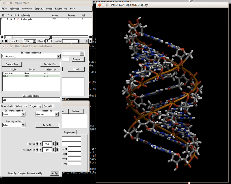
Download the initial PDB structure file (A-dna.pdb) available here. The structure has the sequence d(CGCGAATTCGCG), which is known as the Drew-Dickerson dodecamer, or DDD, and is one of the most famous and studied short oligomers available. Open the file using VMD so you can see the structure that we are going to use for our tutorial.
$ vmd A-dna.pdb
Next we need to generate the topology and the coordinate files for the system so we can run our simulation. We do that using the LEaP module of AmberTools. The recommended force field for nucleic acids (DNA) has the name OL15, which is named after the city of Olomouc where it was developed in the year 2015. A comprehensive review of this force field is available in these set of published articles (link 1 and link 2). Open tleap (we do not need to use the visual interface, so tleap is the terminal version):
$ tleap
Source the force field, which has the name leaprc.DNA.OL15
$ source leaprc.DNA.OL15
As you can see, when the force field loads, there is a line which states what modifications are being loaded. For nucleic acids, it loads:
OL15 force field for DNA (99bsc0-betaOL1-eps-zetaOL1-chiOL4) see http://ffol.upol.cz
Which means that we are loading the ff99bsc0 modifications for the alpha/gamma dihedrals plus the OL1 set of modifications for the epsilon/zeta dihedral and the OL4 modifications for the chi angel. Yes, it is very confusing… but it works. In tleap, if we type the comand list, we can now see all the residues that we have loaded:
> list
DA DA3 DA5 DAN DC DC3 DC5 DCN
DG DG3 DG5 DGN DT DT3 DT5 DTN
parm10
Since the molecule we are using has a negative charge, we load the ions force field so we can use them to net neutralize our system. The current AMBER instruction are designed to load the water model and the ions model recommended:
> source leaprc.water.opc
This will load the water model known as Optimum Point Charge (OPC) and the ion parameters that have been shown to be compatible with that current water model. We now load our DNA structure with the command loadpdb and asign it to the variable dna:
> dna = loadpdb A-dna.pdb
    Loading PDB file: ./A-dna.pdb
    total atoms in file: 758
Check our structure for possible errors:
> check dna
		Checking 'dna'....
     WARNING: The unperturbed charge of the unit: -22.000000 is not zero.
     Checking parameters for unit 'dna'.
     Checking for bond parameters.
     Checking for angle parameters.
     check:  Warnings: 1
     Unit is OK.
The structure has a -22 charge which is expected since we have 22 phosphate groups. At this step we can proceed and add counter ions to neutralize the charge.
> addions dna Na+ 0
This command will add ions to the variabla dna, using Na+ type ions until it reaches a charge of ‘0’. The ions are added close to the negative sites of the molecule. Next, we solvate the system:
> solvateoct dna OPCBOX 9.0
The command solaveoct will create a truncated octahedron periodic cell centered on the variable dna which contains our systems and add explicit water molecules using the OPC water model. The tleap program will add at least 9.0 angstroms of water molecules between the solute (our DNA molecule) and the borders of the box. Around 5336 water molecules should be added.
That is it. Next we generate the topology file and the coordinates file of our system:
> saveamberparm dna dna.prmtop dna.rst7
This will generate a topology and coordinates file using the force field and force field modifications we loaded previously. After this, we quit tleap
> quit
We now have the topology file dna.prmtop that contains all the parameter definitions for each atom in our system and a coordinate file dna.rst7 that has all the xyz coordinates for each atom.
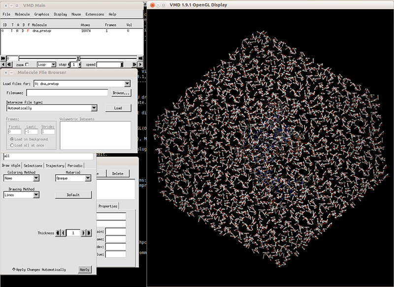
We can check our topology and coordinates file with VMD. Launch VMD and load the topology file dna.prmtop. It will recognize the file as an AMBER7 parm file. Load the file and in the VMD main windows it should display the number of atoms. Next, load the coordinates file dna.rst7 and it should be loaded like an AMBER7 restart file. Hit load and you should be able to see the solvated system.
Close VMD and now we are ready to run minimization and equilibration of our DNA molecule. We will use the following protocols:
| mini.in | heat.in | eq.in |
Minimzing the system with 25 kcal/mol restraints on DNA, 500 steps of steepest descent and 500 of conjugated gradient &cntrl imin=1, ntx=1, irest=0, ntpr=50, ntf=1, ntb=1, cut=9.0, nsnb=10, ntr=1, maxcyc=1000, ncyc=500, ntmin=1, restraintmask=':1-24', restraint_wt=25.0, &end &ewald ew_type = 0, skinnb = 1.0, &end |
Heating the system with 25 kcal/mol restraints on DNA, V=const &cntrl imin=0, ntx=1, ntpr=500, ntwr=500, ntwx=500, ntwe=500, nscm=5000, ntf=2, ntc=2, ntb=1, ntp=0, nstlim=50000, t=0.0, dt=0.002, cut=9.0, tempi=100.0, ntt=1, ntr=1,nmropt=1, restraintmask=':1-24', restraint_wt=25.0, &end &wt type='TEMP0',istep1=0, istep2=5000, value1=100.0,value2=300.0, &end &wt type='TEMP0',istep1=5001, istep2=50000, value1=300.0,value2=300.0, &end &wt type='END', &end |
Equilibrating the system with 0.5 kcal/mol restraints on DNA, during 500ps, at constant T= 300K & P=1ATM and coupling = 0.2 &cntrl imin=0, ntx=5, ntpr=500, ntwr=500, ntwx=500, ntwe=500, nscm=5000, ntf=2, ntc=2, ntb=2, ntp=1, tautp=0.2, taup=0.2, nstlim=25000, t=0.0, dt=0.002, cut=9.0, ntt=1, ntr=1, irest=1, restraintmask=':1-24', restraint_wt=0.5, &end &ewald ew_type = 0, skinnb = 1.0, &end |
First we run mini.in, then heat.in and last eq.in. Remember that these are only examples to setup simulations. For actual research simulations a more thorough minimization and equilibration protocol should be used.
To run mini.in:
$ pmemd -i mini.in -o mini.out -p dna.prmtop -c dna.rst7 -r mini.rst -ref dna.rst7
To run heat.in:
$ pmemd -i heat.in -o heat.out -p dna.prmtop -c mini.rst -r heat.rst -x heat.mdcrd -ref mini.rst
The last step, eq.in:
$ pmemd -i eq.in -o eq.out -p dna.prmtop -c heat.rst -r eq.rst -x eq.mdcrd -ref heat.rst
This equilibration steps will generate a reasonable starting system that we can use for production MD simulation using the input file:
| md.in |
 production
 &cntrl
    imin=0, ntx=5,
    ntpr=1000,ntwr=1000,
    ntwx=1000,ntwe=1000,
    nscm=1000,
    ntf=2, ntc=2,
    ntb=2, ntp=1, tautp=5.0, taup=5.0,
    nstlim=100000, t=0.0, dt=0.002,
    cut=9.0,
    ntt=1,
    irest=1,
    iwrap=1,
    ioutfm=1,
 &end
 &ewald
    ew_type = 0, skinnb = 1.0,
 &end
|
To run the production simulation we use:
$ pmemd -i md.in -o md.out -p dna.prmtop -c eq.rst -r md.rst7 -x md.nc -inf mdinfo
This will run pmemd for 2 nanoseconds, which is just good enough to see the DNA dynamics and conformational changes. The simulation will generate a restart file (md.rst7) and a trajectory file in the binary NetCDF format (md.nc)
Analysis of the trajectory using CPPTRAJ
The program CPPTRAJ developed by Dr. Dan Roe and other collaborators is our main engine to analyze AMBER molecular dynamics simulations. It has a huge array of commands and analysis actions and is also focused on speed. This is very important since we now analyze trajectories no shorter than microsecond time scale, which represents tens of millions of frames. The paper describing CPPTRAJ is D. Roe and T.E. Cheatham, III available at: JCTC link
CPPTRAJ can be run either using an input script or in interactive mode. Using an input script is useful when you want to automate a lot of analysis or when submitting the analysis for a compute cluster, for example. Also, having the script allows you to remember what you did (provenance). The interactive mode is great for doing short, simple analysis and also to look at the extensive integrated help which is often the most up-to-date source of help information for the program.
Our first CPPTRAJ analysis will generate a stripped trajectory and reorient it to the center so we can see the simulation in VMD. Also, it is faster to work with stripped trajectories (that is, without water), siwnce it saves a considerable amount of time and hard disk space.
The input script is:
| process1.cpptraj | |
parm dna.prmtop trajin md.nc autoimage strip :WAT trajout md-nowater.nc netcdf |
Load the corresponding topology file Load the trajectory file Automatically center and image a trajectory with periodic boundaries Strip all residues with the name ‘WAT’ (delete the water molecules) Save the resulting trajectory in NetCDF format. |
Needed files:
dna.prmtop
md.nc
Run CPPTRAJ with the command:
$ cpptraj -i process1.cpptraj
This will run CPPTRAJ, read the input file and execute the analysis.
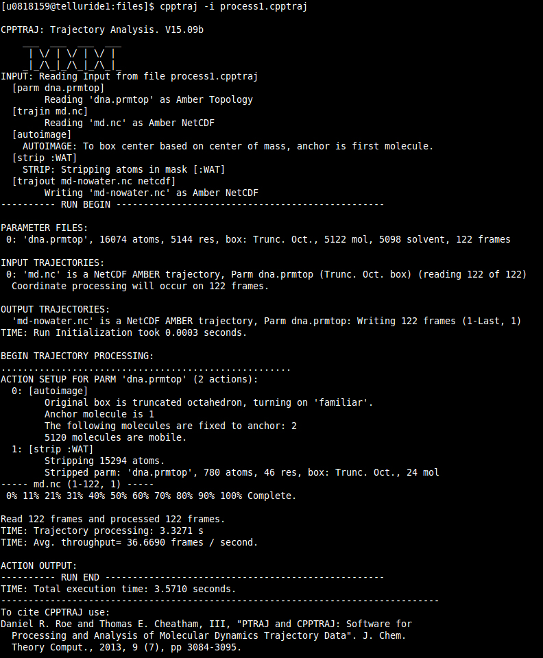
This generates a new trajectory file with the name ‘md-nowater.nc’ which is autoimaged and has no waters. Before we can see the movie in VMD (or chimera), we need a new topology file. This is because our topology file still has waters. To generate a stripped topology file we can use either CPPTRAJ or the python program ‘parmed.py’
We will use parmed.py to demonstrate quickly how it works.
Load the topology in parmed.py
$ parmed.py dna.prmtop
Run the command to strip waters:
> strip :WAT
Save the new topology file:
> parmout dna-nowater.prmtop
Type ‘go’ to run the process:
> go
This reads in the topology file, deletes all the residues with the name WAT and saves a new topology file with the name ‘dna-nowater.prmtop‘
Now we can open our trajectory in VMD:
$ vmd -parm7 dna-nowater.prmtop -netcdf md-nowater.nc
This command will open VMD, load the topology file and load the frames included in the NetCDF file. You must be able to see a big conformational change as the DNA switches from the A- to the B- form configuration.
Now we can do further analysis using CPPTRAJ. We are going to group a bunch of analysis in the same input script. This is faster since the trajectory file will be read only once and with the data loaded, several analysis can be made.
We will perform:
RMSD calculation – this will measure the deviation of the structure over time
Pucker distributions – a measure of the sugar puckers, so we can check the conformational change
Structural parameters – a collection of parameters specific of nucleic acids, specially the helical axis
Needed files: dna.prmtop and md.nc
The CPPTRAJ input for the analysis is:
| process2.cpptraj | |
parm dna-nowater.prmtop

trajin md-nowater.nc

rmsd all first :1-24&!@H= out rmsd-all.agr mass

rmsd notail first :3-10,15-22&!@H= \
       out rmsd-all.agr mass

pucker pucker5 :5@C1' :5@C2' :5@C3' :5@C4' :5@O4' \
       out pucker.agr range360

pucker pucker6 :6@C1' :6@C2' :6@C3' :6@C4' :6@O4' \
       out pucker.agr range360

pucker pucker7 :7@C1' :7@C2' :7@C3' :7@C4' :7@O4' \
       out pucker.agr range360

pucker pucker8 :8@C1' :8@C2' :8@C3' :8@C4' :8@O4' \
       out pucker.agr range360

nastruct resrange 6,7,18,19 naout data_6-7 noheader
|
– Load the corresponding topology file
– Load the trajectory file – Measure the RMSD values and save it to a dataset called ‘all’. Use the first frame as a reference. Measure the residues 1 through 24, but only the atoms that are not H. Save the file as an xmgrace type of file with name rmsd-all.agr. l Use the mass of the atoms for measuring. – Measure the RMSD values and save it to a dataset called ‘notail’. Use the first frame as a reference. Measure the residues 3 through 10 and 15 to 22, but only the atoms that are not H. Save the file as an xmgrace type of file with name rmsd-all.agr. Using the same name as the first measure, will combine the two measurements into a single xmgrace filel Use the mass of the atoms for measuring. – The pucker commands measure the pseudo-pucker rotation around the atoms C1′ through O4′ of residue 5. Data is saved to an xmgrace file called pucker.agr and it will be modified to a 360 degrees range (instead of -180 to +180 degrees). The same command follows but residues 6 through 8. – The nastruct command calculates basic nucleic acids structure parameters. The resrange states that only the base pair 6,7 and 18,19 will be read and will generate a file with the suffix data_6-7. This file will include the shear, stretch, stagger, buckle, propeller, opening HB, major and minor groove measurements for that particular base pair. |
If we open the file ‘rmsd-all.agr’:
$ xmgr rmsd-all.agr
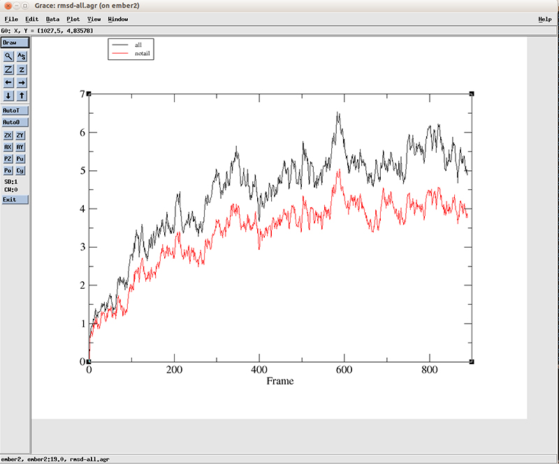
We have two lines, which corresponds to the two datasets we calculated with CPPTRAJ. The blackline is using all the residues and the red line is using residues 3 to 10 and 15 to 22. We can see that a variation of more than 4 angstroms is present at the starting of the simulation for the black line (using all atoms) and a little lower for the red line. After around the frame 400, the values fluctuate between 4.5 and 5.5 angstoms when using all atoms and around 3.5 and 4.5 for the central base pairs. This suggest a big conformational shift early on the simulation which we already saw using VMD.
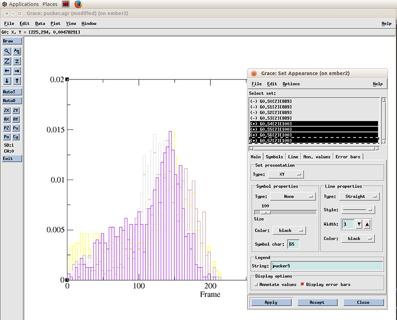
The pucker distribution (file pucker.agr) for residues 5 through 8 looks like this:
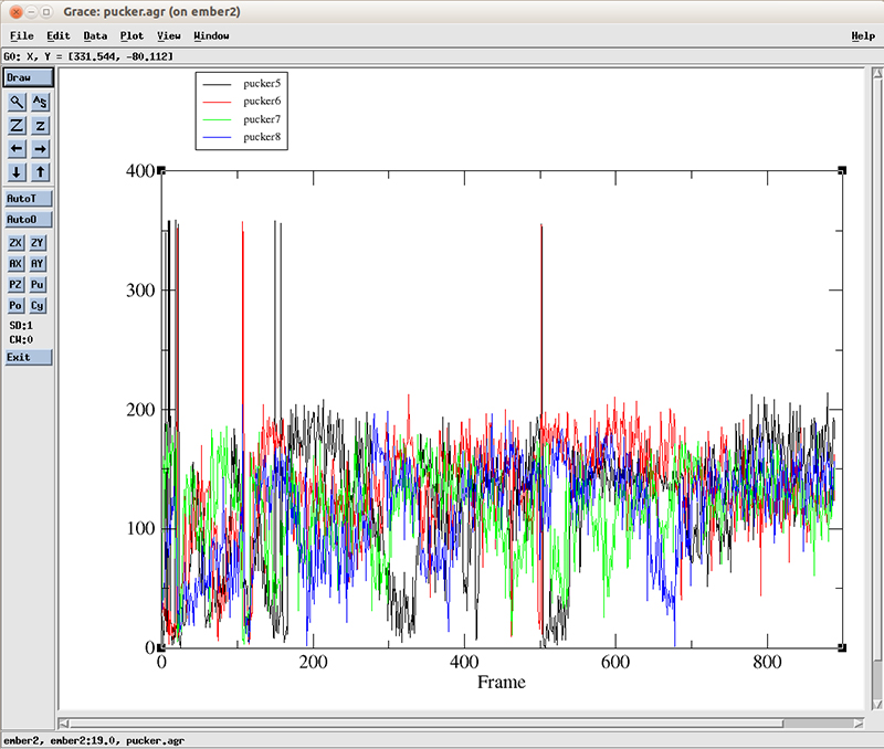
Each line corresponds to the pucker pseudo-rotation angle for residues 5 to 8. At the start of the simulation, we can roughly see more population of values going from 0 to around 100 degrees (which corresponds to a C3′-endo configuration, present in the A-DNA form). After 600 frames, the values cluster between 100 and 200 degrees which corresponds to a C2′-endo configuration present for B-DNA. For details about all these configurations and measurements, we recommend the Nucleic Acids bible which is the Wolfram Saenger book ‘Principles of Nucleic Acid Structure’.
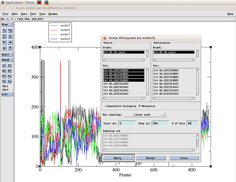
The pucker distribution is easier to differentiate if we calculate the histogram for each residue. In xmgrace, we go to -> Data -> Transformations -> Histograms…
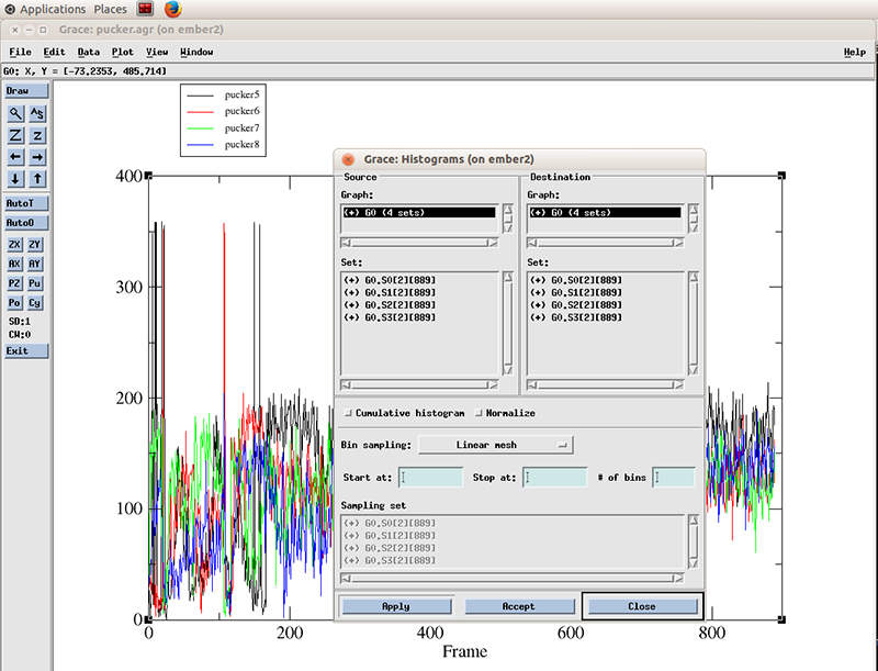
We select all the datasets present (4 because we calculated the pucker distributions for 4 residues). We will calculate a histogram starting at 0 degrees and finish at 360 with 99 bins and normalize it.
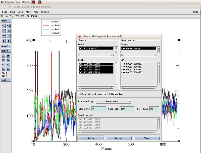
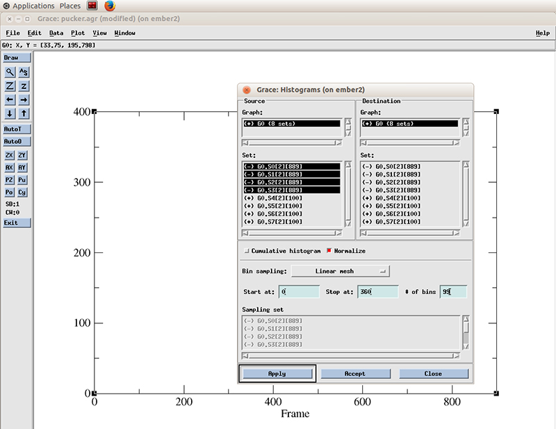
Hit apply. The histograms will be calculated for each dataset.
With the Histograms windows still open, we right click on the highlighted datasets and click hide. This will hide the original values. We have to do that so we can actually see the new generated histogram data.
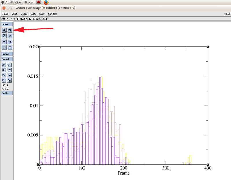
Close the histograms windows and hit the recenter icon to rescale the plot
Go to Plot -> Set Appearance
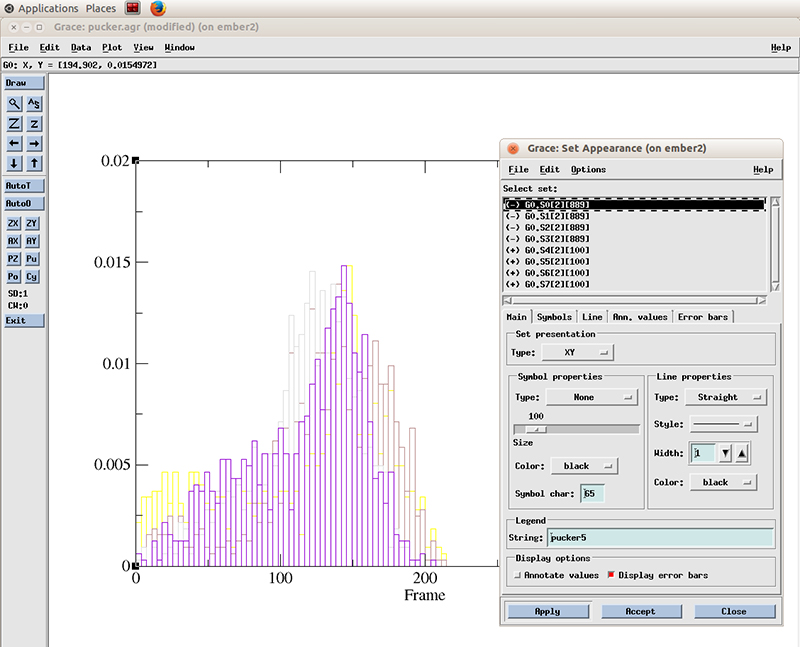
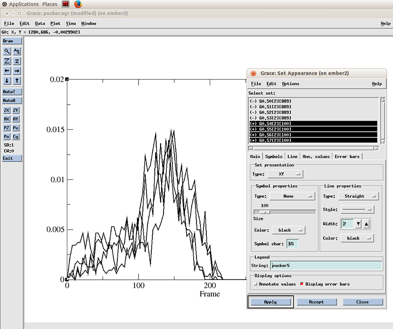
And select the datasets with the plus symbol next to it (+). These are our active (not hidden) datasets. You can simply click the first one and drag the mouse to multi select the 4 datasets.
Select Line properties to Straight, Width to 2 and hit Apply
Now in the Set Appearance window, go to Edit and click on Set different colors.
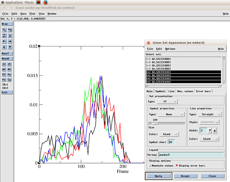
Now we can see more easily that the population of values for the pucker distribution is mainly in the 110 to 180 degrees which corresponds to the C2′-endo configuration. The curves does not appear smooth since we only have ~800 frames of simulation. Extending the simulation will show a nicer distribution.
The nastruct comand will generate 3 files. One with the information for base pairs (BP.data_6-7). The first column is the time frame and each column stands for:
#Frame Base1 Base2 Shear Stretch Stagger Buckle Propeller Opening HB Major Minor
We include here what each column stands for, because since we included the ‘noheader’ keyword in the nastruct command, no header will be written in the output file. Another file generated by nastruct is one with the information of the step parameters between the central base pairs 6,19 and 7,18 (BPstep.data_6-7):
#Frame BP1 BP2 Shift Slide Rise Tilt Roll Twist
and the last one with helical parameters involved in the same base pairs (Helix.data_6-7):
#Frame BP1 BP2 X-disp Y-disp Rise Incl. Tip Twist
Of course one could expand to include more base pairs, but it will require more post processing of the output files. In this case we will see how the helicoidal twist between the central base pairs of our DNA (base pairs 6-19 and 7-18) chain evolve over time.
The file we will use is the BPstep.data_6-7 which has on the last column the twist value. We first have to do a bit of unix-kung-fu to properly format the files. First lets delete the extra blank lines from the CPPTRAJ output file using sed:
$ sed -e '/^$/d' BPstep.data_6-7 > BPstep.data_6-7.new
Then we extract colum 1 (the frame count) and column 9 (the twist value) using awk:
$ awk '{print $1 "\t" $9}' BPstep.data_6-7.new > twist_6-7.dat
Now we can plot the twist value with xmgrace:
$ xmgr twist_6-7.dat
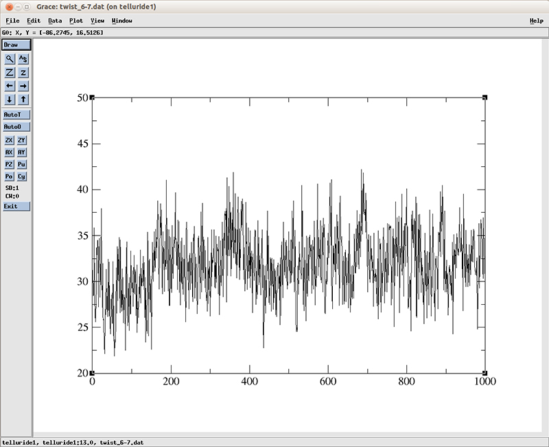
The plot shows an increase on the average twist value around the frame 180 which roughly matches the time on which the RMSD deviation converges. Of course this is only one base pair, it would require further analysis on the rest of the DNA molecule to actually study the entire conversion process between the A-B conformation.