
Introduction to Principal Component Analysis
Principal component analysis with CPPTRAJ
The goal here is to perform principal component analysis (PCA) using CPPTRAJ on two different trajectories of a 36-mer double stranded DNA, d(GCACGAACGAACGAACGC). One of the trajectories was run on GPUs and the other on CPUs with the goal of determining if both technologies sampled the same conformational space of the DNA. The trajectories here are exemplary; the full data is available at: http://amber.utah.edu/DNA-dynamics/GAAC
Papers describing this work:
- R Galindo-Murillo, DR Roe, and TE Cheatham, III. “Convergence and reproducibility in molecular dynamics simulations of the DNA duplex d(GCACGAACGAACGAACGC).” Biochimica Biophys. Acta 1850,1041-1058 (2015). doi: 10.1016/j.bbagen.2014.09.007.[BBAGEN link]
- R Galindo-Murillo, DR Roe, and TE Cheatham, III. “On the absence of intrahelical DNA dynamics on the μs to ms timescale.”
Nature Commun. 5:5152 (2014) doi: 10.1038/ncomms6152.[Nature Commun. link]
Brief Introduction to PCA.
PCA is a technique that can be used to transform a series of potentially coordinated observations into a set of orthogonal vectors called principal components (PCs). One way to think of PCs is that they are a means of explaining variance in the data. If the input data are Cartesian coordinates, then a PC is a means of showing variance in coordinate space. PCA is done in such a way that the first PC shows the largest variance in the data, the second PC shows the second largest and so on. The input to PCA in this example will be the coordinate covariance matrix calculated from the time series of 3D positional coordinates, so the PCs will represent certain modes of motion undergone by the system, with the first PC representing the dominant motion.
One important thing to keep in mind is that while PCA is useful for gaining insight into the dynamics of a system, the actual motion of the system throughout the course of a simulation is almost always a combination of the individual PCs. So while motion along a single PC might show a transition, it is usually not actually how the system undergoes that transition.
Step 1: Calculation of the coordinate covariance matrix
As mentioned above, the input to PCA will be a coordinate covariance matrix. The entries to this matrix are the covariance between the X, Y, and Z components of each atom, so the final matrix will have a size of [3 * # selected atoms] X [3 * # selected atoms]. This means that in order to properly populate this matrix we will need at least as many input frames to calculate the coordinate covariance matrix as we have rows/columns (i.e. 3 * # selected atoms).
The CPPTRAJ script we are going to use is:
#####################################################
# Load two topologies, each with a different        #
# name handler depicted inside []                   #
#####################################################
parm cpu/cpu.prmtop [cpu]
parm gpu/gpu.prmtop [gpu]

#####################################################
# Load two different trajectories                   #
# each with their respective topology.              #
# Each trajectory is 10001 frames long, so          #
# we will have a dataset of 20002 frames long,      #
# the first 10001 frames correspond to the cpu      #
# frames and the from 10002 to 20002, correspond    #
# to the GPU frames.                                #
#####################################################
trajin cpu/cpu.nc parm [cpu]
trajin gpu/gpu.nc parm [gpu]

#####################################################
# Move and translate the coordinates so they will   #
# fit as close as possible to the first frame.      #
# Only fit residues 1 through 36 (the DNA)          #
# and ignore everything that matches the atom 'H'   #
# This means that no hydrogen atoms are going to be #
# part of the fitting.                              #
#####################################################
rms first :1-36&!@H=

#####################################################
# Create an average structure considering all       #
# the loaded frames and save it as a single frame   #
# using the AMBER restart format                    #
#####################################################
average crdset cpu-gpu-average

#####################################################
# CPPTRAJ works with datasets of multiple formats   #
# create a coordinate dataset that refers to the    #
# loaded frames. Call the loaded frames             #
# 'cpu-gpu-trajectories'                            #
#####################################################
createcrd cpu-gpu-trajectories

#####################################################
# Run the commands because we need our reference    #
# structure. With the 'run' command, the            #
# commands so far will run and will generate our    #
# average reference structure with the AMBER        #
# restart format                                    #
#####################################################
run

#####################################################
# Fit our frames, which we named:                   #
# cpu-gpu-trajectories                              #
# to the previously loaded average structure        #
# Always use the same mask                          #
#####################################################
crdaction cpu-gpu-trajectories rms ref cpu-gpu-average :1-36&!@H=

#####################################################
# Calculate coordinate covariance matrix            #
#####################################################
crdaction cpu-gpu-trajectories matrix covar \
name cpu-gpu-covar :1-36&!@H=

#####################################################
# Diagonalize coordinate covariance matrix          #
# Get first 3 eigenvectors                          #
#####################################################
runanalysis diagmatrix cpu-gpu-covar out cpu-gpu-evecs.dat \
vecs 3 name myEvecs \
nmwiz nmwizvecs 3 nmwizfile dna.nmd nmwizmask :1-36&!@H=

#####################################################
# Now create separate projections                   #
# for each set of trajectories                      #
 #####################################################
crdaction cpu-gpu-trajectories projection CPU modes myEvecs \
beg 1 end 3 :1-36&!@H= crdframes 1,10001
crdaction cpu-gpu-trajectories projection GPU modes myEvecs \
beg 1 end 3 :1-36&!@H= crdframes 10002,last

#####################################################
# Make a normalized histogram of the 3              #
# calculated projections                            #
 #####################################################

hist CPU:1 bins 100 out cpu-gpu-hist.agr norm name CPU-1
hist CPU:2 bins 100 out cpu-gpu-hist.agr norm name CPU-2
hist CPU:3 bins 100 out cpu-gpu-hist.agr norm name CPU-3

hist GPU:1 bins 100 out cpu-gpu-hist.agr norm name GPU-1
hist GPU:2 bins 100 out cpu-gpu-hist.agr norm name GPU-2
hist GPU:3 bins 100 out cpu-gpu-hist.agr norm name GPU-3

#####################################################
# Run the analysis                                  #
# ** cross-fingers **                               #
#####################################################

run

#####################################################
#####################################################
# DELETE EVERYTHING AND START FRESH                 #
#####################################################
#####################################################
clear all


#####################################################
# Visualize the fluctuations of the eigenmodes      #
# Read the file with the eigenvectores              #
#####################################################
readdata cpu-gpu-evecs.dat name Evecs


#####################################################
# Load a topology                                   #
# This is necesary to create a new topology         #
# that will match the read in eigenmodes
#####################################################
parm cpu/cpu.prmtop
parmstrip !(:1-36&!@H=)
parmwrite out cpu-gpu-modes.prmtop

#####################################################
# Create a NetCDF trajectory file with the          #
# modes of motion of the first PCA                  #
#####################################################
runanalysis modes name Evecs trajout cpu-gpu-mode1.nc \
pcmin -100 pcmax 100 tmode 1 trajoutmask :1-36&!@H= trajoutfmt netcdf


#####################################################
# Now you can open the files:                       #
# cpu-gpu-modes.prmtop                              #
# cpu-gpu-modes.nc                                  #
# in Chimera / VMD and watch the movie              #
# which shows the first mode of motion              #
#####################################################
As the trajectories may not have the same number of atoms, we need to load up the topology file (prmtop) information for each. We assign a tag or name for each with the name handler [name] functionality.
parm cpu/cpu.prmtop [cpu]
parm gpu/gpu.prmtop [gpu]
The topology file “cpu/cpu.prmtop” can now be referred to by ‘[cpu]’ instead of the full file name. With the topologies loaded, we now want to load up the trajectories each with their respective topologies. In this example, each trajectory is 10001 frames long so our combined data set will be 20002 frames, the first 10001 frames correspond to the cpu frames and the from 10002 to 20002, correspond to the GPU frames.
trajin cpu/cpu.nc parm [cpu]
trajin gpu/gpu.nc parm [gpu]
Now if we were just to calculate the coordinate covariance matrix from the raw trajectory data, we will not only capture internal motion, but also the global rotation and translation of the system. Since in this instance we are interested in only internal dynamics, we need to remove the rotational/translational motion, which we will accomplish by performing a coordinate RMS best-fit to a reference structure, which in our case will be the averaged coordinates. To generate the average coordinates we first put the frames in a common reference by RMS fitting to the first frame using all atoms of the DNA (residues 1-36) except the hydrogen atoms.
rms first :1-36&!@H=
We then create an average structure over the entire set of frames loaded and save the coordinates as ‘cpu-gpu-average’, which can be subsequently
used as a reference structure. Note that if we wanted to we could write the averaged coordinates out to a file in any format CPPTRAJ supports as well.
average crdset cpu-gpu-average
CPPTRAJ has the notion of “data sets” which can be of multiple formats. Here we create a coordinate dataset that will save all of the input frames.
This allows us to act on the entire set later without have to re-read in the trajectories from disk. We refer to the loaded frame coordinate dataset as: cpu-gpu-trajectories.
createcrd cpu-gpu-trajectories
The commands above will generate the average structure which we want to use as a reference. To run the above now, without exiting the program, we input the run command.
run
Now we have generated the averaged coordinates, ‘cpu-gpu-average’, as well as saved the frames from the input trajectories. Now we can RMS-fit the saved trajectory frames to the averaged coordinates to remove global rotational/translational motion. This is done using the crdaction command.
crdaction cpu-gpu-trajectories rms ref cpu-gpu-average :1-36&!@H=
Now we use the matrix command to generate the coordinate covariance matrix, which we will name ‘cpu-gpu-covar’:
crdaction cpu-gpu-trajectories matrix covar \
  name cpu-gpu-covar :1-36&!@H=
Note that the backslash ‘\‘ character can be used to continue a line; this is useful for making complicated input more readable.
Step 2: Calculate principal components and coordinate projections
Now that we have the matrix, we can obtain PCs by diagonalizing it; this will give us the eigenvectors (i.e. the PCs) and the eigenvalues (i.e. the “weight” of each PC). To start, we will obtain the first three eigenvectors:
runanalysis diagmatrix cpu-gpu-covar out cpu-gpu-evecs.dat \
    vecs 3 name myEvecs \
    nmwiz nmwizvecs 3 nmwizfile dna.nmd nmwizmask :1-36&!@H=
The runanalysis command tells cpptraj to run ‘diagmatrix‘ immediately instead of adding it to the Analysis queue. The nmwiz and related keywords generate output which can be used to visualize principal component data with the ‘nmwiz’ plugin for VMD.
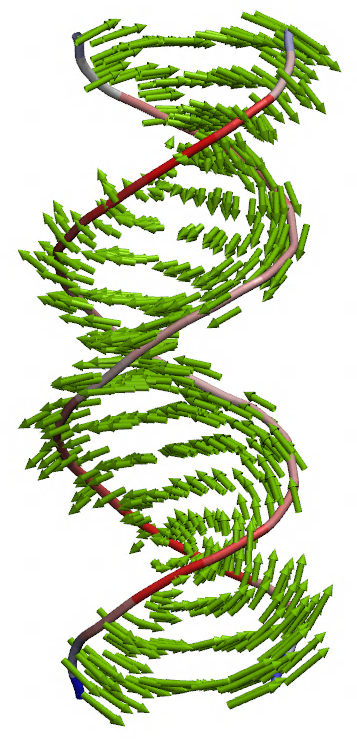
Once this command has completed the file ‘cpu-gpu-evecs.dat’ and the data set ‘myEvecs’ will contain the eigenvectors (PCs) and eigenvalues (this data is referred to collectively as “eigenmode data”). It is often useful to write these out to a file as they can be read back in later for further analysis. We can now project the trajectory coordinates along PCs to see how much the coordinates of each frame “match up” along each principal component. We can do this for the frames from the original individual trajectories, which will essentially allow us to compare how well the motions from each individual trajectory match.
Note that it is critical that the frames used for projection are the same ones used to generate the coordinate covariance matrix.
In this case the saved frames in memory can be used. It is also necessary that the same atom mask that was used to generate the matrix is used for projection.
crdaction cpu-gpu-trajectories projection CPU modes myEvecs \
  beg 1 end 3 :1-36&!@H= crdframes 1,10001
crdaction cpu-gpu-trajectories projection GPU modes myEvecs \
  beg 1 end 3 :1-36&!@H= crdframes 10002,last
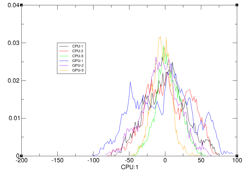
In this case the projections from the cpu trajectories are named ‘CPU’ and the projections from the gpu trajectories are named ‘GPU’. Once this data is generated, we can make normalized histograms of the three calculated projections from each trajectory with hist analysis commands, followed by the run command to actually do the work!
hist CPU:1 bins 100 out cpu-gpu-hist.agr norm name CPU-1
hist CPU:2 bins 100 out cpu-gpu-hist.agr norm name CPU-2
hist CPU:3 bins 100 out cpu-gpu-hist.agr norm name CPU-3

hist GPU:1 bins 100 out cpu-gpu-hist.agr norm name GPU-1
hist GPU:2 bins 100 out cpu-gpu-hist.agr norm name GPU-2
hist GPU:3 bins 100 out cpu-gpu-hist.agr norm name GPU-3

run
The data set indices (e.g. ‘:1’) refer to the principal components, so that ‘CPU:1’ is the first principal component from CPU etc.
Step 3: Visualizing principal components
Now that this phase of the analysis has been completed, we can issue the clear all command to get rid of all stored data so we can do further analysis with a “clean slate”.
clear all
Our next step is to visualize the fluctuations of the eigenmodes. To do this, we read in the generated file with the eigenvectores using the readdata command.
readdata cpu-gpu-evecs.dat name Evecs
Load up a topology and modify it so that it will match how the coordinate covariance matrix (and the subsequent eigenvectors) were calculated:
parm cpu/cpu.prmtop
parmstrip !(:1-36&!@H=)
parmwrite out cpu-gpu-modes.prmtop
Create a NetCDF pseudo-trajectory file of motion along the first PC. The min and max values can be chosen by looking at the histogram of the PC projection.
runanalysis modes name Evecs trajout cpu-gpu-mode1.nc \
  pcmin -100 pcmax 100 tmode 1 trajoutmask :1-36&!@H= trajoutfmt netcdf
Now you can open the files in Chimera / VMD and watch the movie of the first mode of motion!