Calculate states between a small molecule and a receptor
You want to calculate how much time is spent in a particular conformation or state from a simulation between a small molecule and a receptor.
The calcstate command can follow multiple geometric datasets (like those generated by the distance and angle commands) and assign a specific pre-defined state when the criteria matches. To illustrate this, we will use a simulation of a small copper-based compound (Cu[acethyl-acetonate][4,7-dimethyl-phenanthroline]) and the interaction with a 12-mer DNA.
The simulation shows how the ligand explores the minor groove of the DNA as it closes into an AT base pair and eventually pushes the base pair apart, breaking the Watson-Crick pairing. The ligand then gets inserted into the resulting cavity and stays in that pocket for the remaining of the simulation. The topology and the trajectory file of the shown simulation are available here and here.
We want to know how these process develops over time and how much time a particular state is populated. We will define three states: Groove Binding, Partial intercalation and Intercalation. We will define each state using three values, two distance related and one angle related. The first value will be the distance between the ligand (residue ID 25) and the top and bottom base-pairs that form the binding pocket (residues 4,6,19 and 21). The second set of values will be the distance between the AT base-pair that breaks the Watson-Crick pairing and shifts toward the major groove to allow the ligand to move inside the DNA. This will be a distance measure of the center of mass between residues 5 and 20. The third geometric value will be an angle measurement between the ligand (:25), the top base pair in the cavity (:4,21) and the bottom base pair in the cavity (:6,19). Using these three geometric values, we can define our three states.
- Groove binding. This state will be considered when the ligand is between 8 and 17 angstroms of the base-pairs that form the binding cavity (:4,5,19,21); will have a distance between 0 and 12 angstroms of residues :5 and :20 and the angle between the ligand and the binding pocket base-pairs between 0 and 25 degrees.
- Partial Intercalation. This state will be considered when the ligand is between a distance of 5 and 16 angstroms of the cavity base-pairs, a distance of 10 and 14 angstroms between the base-pair :5,20 and an angle between 26 and 95 degrees.
- Intercalation. This state will be considered when the ligand is between a distance of 0 and 4 angstroms of the residues that form the binding pocket; a distance between 14 and 20 angstroms of the base-pair that is broken during intercalation and an angle between the ligand and the center of mass of the residues that form the binding pocket of 95 and 200 degrees.
The CPPTRAJ input file for this look like:
parm vacuo.parm7
trajin vacuo.nc 1 lastframe 1

distance d1 :25 :4,6,19,21 out d1.dat
distance d2 :5 :20 out d2.dat
angle a1 :4,21 :25 :6,19 out a1.dat

calcstate \
state Groove,d1,8,17,d2,0,12,a1,0.25 \
state Partial,d1,5,16,d2,10,14,a1,26,95 \
state Intercalation,d1,0.4,d2,14,20,a1,95,200 \
name DDD \
out calcstate.svt.dat \
curveout calcstate.curve.agr \
stateout calcstate.states.dat \
transout calcstate.trans.dat \
countout calcstate.count.dat
From the example, you can see that we define each state with the state keyword, then the name for the state, then the name of the data set and the minimum/maximum values to accept for each state. For example, the line:
state Partial,d1,5,16,d2,10,14,a1,26,95
translates to: create a state with the name Partial, read the distance of the d1 dataset calculated previously and consider a minimum of 5 and a maximum of 16 for this data set. Then, read the dataset d2 and consider a minimum of 10 and a maximum of 14 and also consider the dataset a1 with a minimum of 26 and a maximum of 95. The values for each d1, d2 and a1 datasets have to be within these ranges to be considered in the Partial state.
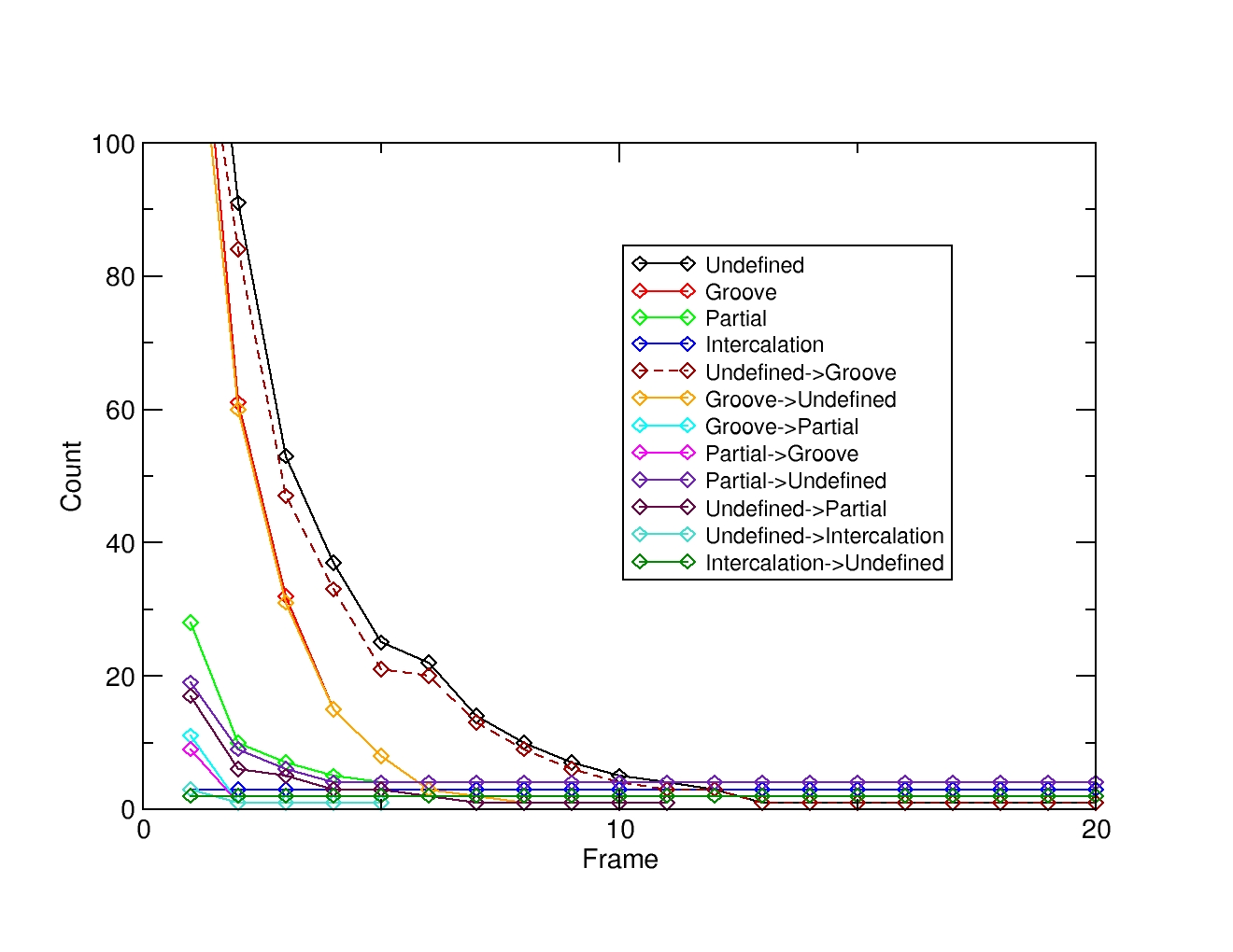
Running this command will generate the files: calcstate.svt.dat, calcstate.curve.agr, calcstate.states.dat, calcstate.trans.dat and calcstate.count.dat. Each with different information. The calcastate.count.dat shows the fraction of each state regarding the total frames:
#Index   DDD[Count]   DDD[Frac]   DDD[Name]
-1       432          0.2159      Undefined
0        264          0.1319      Groove
1        505          0.2524      Partial
2        800          0.3998      Intercalation
This will show that for 21% of the simulation, the system is in an undefined state where the ligand do not match any of the criteria we defined in the CPPTRAJ command. The ligand spends 13% in the Groove state, 25% in the Partial state and 39% in the Intercalation state.
Plotting the file named ‘calcstat.curve.agr’ will show the state lifetime and transition curves for each transition. For our particular case we can see that all the previously defined states will visit an undefined state as seen above. We can also deduce that there is a balance between the groove state and an undefined state that could be further investigated in detail.